Overview
In part one of a four-part series, we are going to set up and walkthrough the Kedro framework. Kedro is an open-source Python framework that provides you with scaffolding to ensure your data projects adhere to software-engineering best practices. In turn, this makes your project reproducible and robust to requirement changes.
Introduction
In this post we are going to talk about and walkthrough using the Kedro framework. To keep things simple, we are going to use a clean dataset provided by the National Oceanic and Atmospheric Association (NOAA) that measures the monthly temperature changes across twelve Brazilian cities. You can download the dataset off of Kaggle. We are going to keep things as simple as possible and only go over the key components of a Kedro project which include:
- Creating a Kedro project
- Defining a data catalog
- Creating a Kedro pipeline
- Integrating Kedro plugins
If you want to learn how to use Kedro’s more advanced features check out the official documention.
Getting Started
Let’s start off by creating a clean environment. We are going to use Conda in this example but you can you whatever virtual environment you prefer. After installing Anaconda or Miniconda, you can create a new environment by executing the following command in your terminal:
# Creates a new virtual environment
conda create -c conda-forge -n my_new_environment python=3.12 -y
The argument -c conda-forge tells conda to put the conda-forge repository at a higher priority over the default repository. We also installed python version 3.12 in this new environment. Now that we have a clean environment we need to install Kedro into that environment. Activate your new environment and install Kedro with:
# Installs kedro
pip install -U kedro==0.19.11
You can verify your installation by executing:
# Displays installed kedro version and extensions
kedro info
Creating a New Kedro Project
Now that we have Kedro installed, we need to create a new Kedro project. You can use the Kedro command-line interface (CLI):
# Creates a new Kedro project
kedro new
You will be prompted to pick a name for your project. Let’s call our project Climate-Brazil. Next, you will be prompted to select the Kedro tools you want to utilize. For this project, let’s go with 1, 3, 5, 7 which corresponds to Linting, Logging, Data Folder, and Kedro-Viz. Once you have created your project, you’ll notice that Kedro created a project directory, using the project name we selected, with subdirectories and files that serve as the scaffolding of your project.
Note that there are some files in the image below that you won’t have at this moment. These will be added/generated as you continue through this walkthrough.
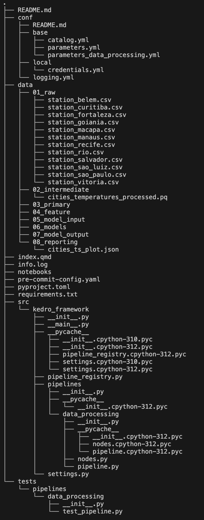
Kedro Project Structure
Let’s briefly walkthrough the 5 subdirectories that Kedro created for us.
conf: This directory contains your project configurations. These can be things from API/Database credentials to Model parameters. This is also where you can create multiple project environments likeDevandProd.data: This directory is where you will store your data and your project artifacts.notebooks: This directory is where you can interactively develop your project before creating modular nodes and pipelinessrc: This directory is where you will put your source code defined as nodes and chained together into pipelinestests: This directory is where you will write your unit tests
I know that was really brief but don’t worry we will learn more specifics as we develop the project.
Declare Project Dependencies
Now that we have a project created, let’s add any packages that our project will depend on. In the root of our project directory Kedro created a requirements.txt file for us. Kedro will add some dependencies into the file by default but we will need some additional packages for our project. We are going to need polars, plotly, and pre-commit so let’s modify requirements.txt to contain the following:
# ./requirements.txt
ipython>=8.10
jupyterlab>=3.0
kedro-datasets>=3.0
kedro-viz>=6.7.0
kedro[jupyter]~=0.19.11
notebook
pre-commit~=3.8.0
polars~=1.22.0
pyarrow~=19.0.1
plotly~=5.24.1
openpyxl~=3.1.5
Now that we have declared our dependencies, let’s go ahead and install them into our environment.
pip install -r requirements.txtDefining a Data Catalog
All Input/Output (IO) operations are defined in a data catalog, when using Kedro. This allows you to declaratively define your data sources whether they are stored as local files, or stored remotely in a SQL/NoSQL database, or just in some form of remote storage like S3.
In our simple example, all the data are stored locally. Therefore, we don’t need to define any credentials to access the data. However, in practice it is likely that you need to access data from a database or cloud storage. In that case, you would define your credentials in /conf/local/credentials.yml.
Before we edit our catalog, go ahead and download the data to /data/01_raw/. You can get the data files from Kaggle.
We declare our base catalog by modifying /conf/base/catalog.yml. The base catalog will be inhereted by all other Kedro enviornments you create. For example, if you create a dev environment you don’t need to repeat the catalog entries that are in /conf/base/catalog.yml inside of /conf/dev/catalog.yml.
If you declare a catalog entry in /conf/dev/catalog.yml that shares the same key as an entry in /conf/base/catalog.yml you will override the base catalog when you are working in the dev environment.
There are several ways that we can add our data to the catalog. The simplest way is to define one entry for each Brazilian city:
#/conf/base/catalog.yml
belem_dataset:
  type: polars.LazyPolarsDataset
  file_format: csv
  filepath: data/01_raw/station_belem.csv

curitiba_dataset:
  type: polars.LazyPolarsDataset
  file_format: csv
  filepath: data/01_raw/station_curitiba.csv

# Rest of the cities follow-suit
If you have a lot of cities it can get really tedious. Luckily, Kedro has a feature called Dataset Factories that assist you in reducing repeated code in your data catalog. We can declare all of our cities with one block like this:
#/conf/base/catalog.yml
# Dataset Factory
"{city}_dataset":
  type: polars.LazyPolarsDataset
  file_format: csv
  filepath: data/01_raw/station_{city}.csv
Kedro is smart enough that during runtime it will use Regex to match {city} to the corresponding dataset city. Finally, the approach we will use is to declare the data as a PartitionedDataset. You can think of each Brazilian city as a partition of the entire dataset that would be composed of all the Brazilian cities. Kedro will return a dictionary object with each file’s name as the key and the load method as the corresponding value.
Note that when using a PartitionedDataset the data is loaded lazily. This means that the data is actually not loaded until you call the load method. This prevents Out-Of-Memory (OOM) errors if your data can’t fit into memory.
We can declare our data as a PartitionedDataset like this:
# /conf/base/catalog.yml
cities_temperatures:
  type: partitions.PartitionedDataset
  path: data/01_raw/
  dataset:
    type: polars.LazyPolarsDataset
    file_format: csv
Now we can load our dataset by simply starting up a Kedro session (Kedro does this for you) and calling catalog.load("cities_temperatures"). You can even work with the data interactively in a jupyter notebook. Kedro automatically loads the session and context when you run kedro jupyter lab on the command-line. This means that once the jupyter kernel is running you already have your catalog object loaded in your environment.
Creating a New Kedro Pipeline
Typically, once you have defined your data catalog you’d want to work interactively on your cleaning and wrangling your data into a usable format. As mentioned earlier you can do that using kedor jupyter lab. Once you have your processing/modeling/reporting code in check you should write modular functions that when chained together would constitute a pipeline. That could be a data processing pipeline, a machine learning pipeline, a monitoring pipeline, etc… This is where Kedro pipelines come in to play. We can create a new pipeline using the Kedro CLI by executing:
kedro pipeline create data_processingKedro will create the structure for your new pipeline in /src/climate_brazil/pipelines/data_processing. We will define all your modular code inside of /src/climate_brazil/pipelines/data_processing/nodes.py and then we will declare our pipeline inside /src/climate_brazil/pipelines/data_processing/pipeline.py. Let’s start with the nodes.
Each of our Brazilian cities dataset is in a wide format where we have years across the rows and the months within that year across the columns. We need to merge all of our cities together and unpivot the data so that we are in long format where both year and month are across the rows. The following function does what we just described:
# /src/climate_brazil/pipelines/data_processing/nodes.py
def process_datasets(partitioned_dataset: dict) -> pl.DataFrame:
    """
    Combine all cities into one dataframe and unpivot the data into long format
    ---
    params:
        partitioned_dataset: Our data partiotioned into key (filename) value(load method) pairs
    """
    # Missing values encoding
    mv_code = 999.9

    # Add a city column to each partiotion so that when we merge them all together we can identify each city
    datasets = [
        v().with_columns(city=pl.lit(re.findall(r"(?<=_).*(?=\.)", k)[0]))
        for k, v in partitioned_dataset.items()
    ]

    df_merged = pl.concat(datasets)

    df_processed = (
        df_merged.drop("D-J-F", "M-A-M", "J-J-A", "S-O-N", "metANN")
        .rename({"YEAR": "year"})
        .collect()  # Need to collect because can't unpivot a lazyframe
        .unpivot(
            on=[
                "JAN",
                "FEB",
                "MAR",
                "APR",
                "MAY",
                "JUN",
                "JUL",
                "AUG",
                "SEP",
                "OCT",
                "NOV",
                "DEC",
            ],
            index=["city", "year"],
            variable_name="month",
            value_name="temperature",
        )
        .with_columns(
            pl.col("month")
            .str.to_titlecase()
            .str.strptime(dtype=pl.Date, format="%b")
            .dt.month()
        )
        .with_columns(
            date=pl.date(year=pl.col("year"), month=pl.col("month"), day=1),
        )
        .with_columns(
            pl.when(
                pl.col("temperature")
                == mv_code  # This is how missing data is coded in the dataset
            )
            .then(None)
            .otherwise(pl.col("temperature"))
            .name.keep(),
            pl.col("city").str.to_titlecase(),
        )
        .drop("year", "month")
    )
    return df_processed
Let’s also define a function that will plot our time series data.
def timeseries_plot(processed_dataframe: pl.DataFrame) -> go.Figure:
    """
    Plots each Brazilian city temperature time series
    """
    fig = go.Figure()
    for city in processed_dataframe.select("city").unique(maintain_order=True).to_series():
        fig.add_trace(
            go.Scatter(
                x = processed_dataframe.filter(pl.col("city")==city).sort('date')['date'],
                y = processed_dataframe.filter(pl.col("city")==city).sort('date')['temperature'],
                name = city,
                hovertemplate="<b>Date</b>: %{x}<br><b>Temperature</b>: %{y}"
            )
        )
    fig.update_layout(
        title = "Temperature Measurements of Brazilian Cities",
        xaxis=dict(
        title = "Date",
        rangeselector=dict(
            buttons=list([
                dict(count=1,
                     label="1y",
                     step="year",
                     stepmode="backward"),
                dict(count=5,
                     label="5y",
                     step="year",
                     stepmode="backward"),
                dict(count=10,
                     label="10y",
                     step="year",
                     stepmode="backward"),
                dict(step="all", label="All")
            ])
        ),
        rangeslider=dict(
            visible=True
        ),
        type="date",
        rangeselector_font_color='black',
        rangeselector_activecolor='hotpink',
        rangeselector_bgcolor='lightblue',
    ),
        yaxis=dict(
            title = "Temperature in Celsius"
        )
    )
    return fig
This will produce the following figure:
Now that we have defined our nodes, let’s see how we can chain them together into a simple pipeline. We define our data processing pipeline in the pipeline.py file that Kedro creates for us in the data_processing directory.
# /src/climate_brazil/pipelines/data_processing/pipeline.py
from kedro.pipeline import node, Pipeline, pipeline  # noqa
from .nodes import process_datasets, timeseries_plot

def create_pipeline(**kwargs) -> Pipeline:
    return pipeline([
        node(
            func=process_datasets,
            inputs=dict(partitioned_dataset = "cities_temperatures"),
            outputs="cities_temperatures_processed",
            name="process_datasets"
        ),
        node(
            func=timeseries_plot,
            inputs=dict(processed_dataframe = "cities_temperatures_processed"),
            outputs="cities_ts_plot",
            name="timeseries_plot"
        ),
    ])
Notice that the input to the process_datasets function is the name that we chose for our dataset when we defined it inside of our catalog. Also note that we are choosing to name the output from the process_datasets function as cities_temperatures_processed and we are passing that as the input to the function timeseries_plot.
Kedro automatically infers the dependencies of your pipeline and will run it in an order that may not be the same order as you defined.
Before we move on to the next section, it is important to know that both our outputs will be MemoryDatasets this mean that they will only exist while the Kedro session is still active. In order to persist the outputs we need to add them to our catalog.
# conf/base/catalog.yml
# Raw data ---------------------------------------
cities_temperatures:
  type: partitions.PartitionedDataset
  path: data/01_raw/
  dataset:
    type: polars.LazyPolarsDataset
    file_format: csv

# Processed data ---------------------------------------
cities_temperatures_processed:
  type: polars.EagerPolarsDataset
  file_format: parquet
  filepath: data/02_intermediate/cities_temperatures_processed.pq

cities_ts_plot:
  type: plotly.JSONDataset
  filepath: data/08_reporting/cities_ts_plot.json
We are going to store our processed data locally as a parquet file and our figure as a json file. Great, we are now ready to run our pipeline!
Running a Kedro Pipeline
To run the data processing pipeline we just defined you can execute:
kedro runThat will run all your defined pipelines in the order that you defined them and since we only have one pipeline you will run the data processing pipeline. Okay, so how do we run a specific pipeline? For that you can use:
kedro run --pipeline data_processingKedro also allows you to run specific nodes. For example, if we just wanted to process the data without generating a plot we could run:
kedro run --nodes process_datasetsWhere process_datasets is the name we gave the node when we defined the pipeline.
Kedro is very flexible and allows you to run in a variety of options. You can checkout the Kedro run documentation for more information.
Pipeline Graphs with Kedro-Viz
When we created a new Kedro project earlier, we told kedro to add to our dependencies the kedro-viz plugin. This plugin allows you to visualize your pipeline or pipelines as a graph. To view the simple pipeline we built earlier you can execute at the command-line the following:
kedro viz runYour browser should automatically launch and you will be greeted by the following screen.
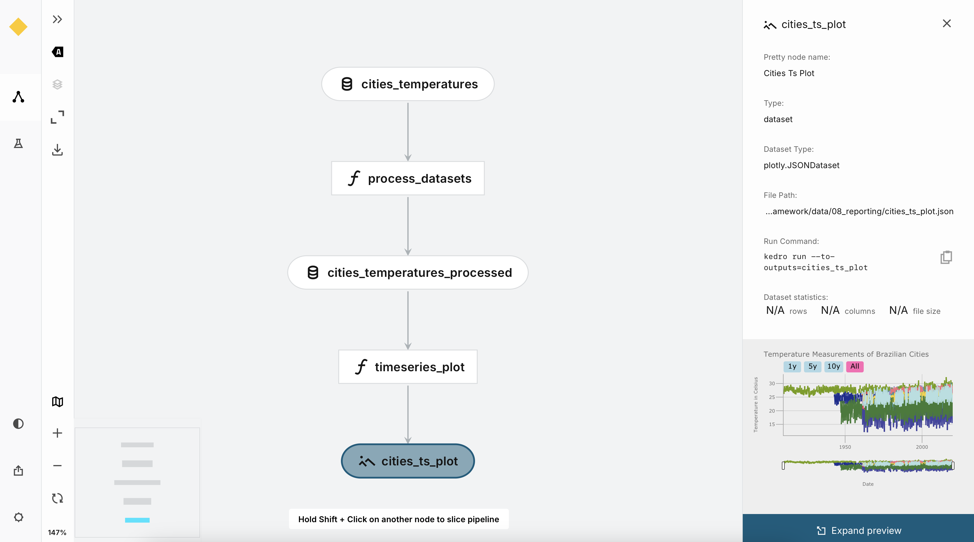
Our simple example doesn’t do Kedro-Viz justice. In practice, you’ll have many datasets coming from disparate sources that will require more complex processing and joining. In such a scenario, being able to see the lineage and dependencies of your data becomes very useful. Kedro-Viz is interactive in that you can optionally preview the data, you can view static or interactive figures, and you can view the code of the nodes all in the user interface. I recommend that you try this plugin for you next project!
Source Control & Pre-Commit
I am sure that everyone reading this already understands the importance of source/version control, so I will keep this breif. When we created our project Kedro was nice enough to create a .gitignore file and .gitkeep files. The .gitignore file makes sure that you don’t accidentally commit any data or any credentials that you store in conf/local/credentials.yml to a remote repository. Kedro does not, unfortunately, set up any pre-commit configuration so you need to do that manually. Here is an example of a pre-commit configuration that includes linting with ruff checking your codebase for missing docstrings with interrogate and stripping out any confidentiat data from notebooks with nbstripout.
# .pre-commit-config.yaml
repos:
  - repo: https://github.com/astral-sh/ruff-pre-commit
    # Ruff version.
    rev: v0.11.2
    hooks:
      # Run the linter.
      - id: ruff
        types_or: [ python, pyi ]
        args: [ --fix ]
      # Run the formatter.
      - id: ruff-format
        types_or: [ python, pyi ]
  - repo: https://github.com/econchick/interrogate
    rev: 1.7.0
    hooks:
    - id: interrogate
      args: [--config=pyproject.toml]
      pass_filenames: false
  - repo: https://github.com/kynan/nbstripout
    rev: 0.7.1
    hooks:
      - id: nbstripout
You also need to specify interrogate’s configuration within pyproject.toml you can add the following at the bottom of your file:
[tool.interrogate]
ignore-init-method = false
ignore-init-module = false
ignore-magic = false
ignore-semiprivate = false
ignore-private = false
ignore-property-decorators = false
ignore-module = false
ignore-nested-functions = false
ignore-nested-classes = false
ignore-setters = false
ignore-overloaded-functions = false
fail-under = 80
exclude = ["tests", "docs", "build", "src/climate_brazil/__main__.py"]
ext = []
verbose = 2
quiet = false
whitelist-regex = []
color = true
omit-covered-files = false
After you’re done setting up your configuration you need to initialize a local git repository and install your pre-commit configurations.
git init
pre-commit install
Wonderul, we are all set now with source control and mitigating the possibility of commiting anything confidential to your repository.
Running Pipelines in Containers
We can also run the pipeline we just built inside of a container. Kedro maintains the kedro-docker plugin which facilitates getting your Kedro project running inside a container.
While the plugin is named kedro-docker you can use it with other containerization frameworks such as Podman
First, we need to install the plugin. You can add the following to your ./requirements.txt file:
kedro-docker~=0.6.2Then execute:
pip install kedro-docker~=0.6.2With the plugin installed, Kedro will generate a Dockerfile, .dockerignore, and .dive-ci that corresponds to your Kedro project by executing:
kedro docker initMake sure you Docker Engine is running otherwise the previous step will fail.
Let’s take a look at the generated Dockerfile:
#./Dockerfile
ARG BASE_IMAGE=python:3.9-slim
FROM $BASE_IMAGE as runtime-environment

# update pip and install uv
RUN python -m pip install -U "pip>=21.2"
RUN pip install uv

# install project requirements
COPY requirements.txt /tmp/requirements.txt
RUN uv pip install --system --no-cache-dir -r /tmp/requirements.txt && rm -f /tmp/requirements.txt

# add kedro user
ARG KEDRO_UID=999
ARG KEDRO_GID=0
RUN groupadd -f -g ${KEDRO_GID} kedro_group && \
    useradd -m -d /home/kedro_docker -s /bin/bash -g ${KEDRO_GID} -u ${KEDRO_UID} kedro_docker

WORKDIR /home/kedro_docker
USER kedro_docker

FROM runtime-environment

# copy the whole project except what is in .dockerignore
ARG KEDRO_UID=999
ARG KEDRO_GID=0
COPY --chown=${KEDRO_UID}:${KEDRO_GID} . .

EXPOSE 8888

CMD ["kedro", "run"]
Kedro will automatically assume that you want to run all your pipelines (or your defualt pipeline) but you can, quite easily, change the specified command in the generated docker file.
Now that we have a Dockerfile and .dockerignore we can build our image.
kedro docker buildFinally, you can run your pipeline from within the container by either using your normal docker-cli commands or you can use the kedro-docker plugin and execute:
kedro docker runSummary
In this post we walked through using the Kedro framework and learned how to follow software engineering best practices that ensure that your projects are reproducible, modular, and easy to maintain as a project matures. We learned about the data catalog, how to define nodes and subsequently linking nodes together to build pipelines. We then looked at a couple Kedro plugins like kedro-viz and kedro-docker that expanded the functionality of our project. We also talked about and walked through good practices to follow when implementing source control with git and pre-commit. All this in just part one of our series! We have a long ways to go still but I hope you are excited for what comes next.
Coming Next
If you use a popular/mainstream machine learning framework like PyTorch, TensorFlow, Scikit-Learn, or XGBoost then reproducibility and scalability are quite easy because you’ll typically find that most MLOPs and distributed frameworks natively support these tools. What do you do if you have a custom solution? Let’s say you are using a probabilistics programming language like Stan or PyMC and there isn’t native support for these tools. Well, that is what we are going to do in the following parts of this series. In part two we will fit a time series model using PyMC and talk about how to use ModelBuilder from pymc-extras to build a production ready model. I hope to see you there!